YCSB is a well known benchmark that was devised by a group at Yahoo! Research led by Brian F. Cooper. It came about because the proliferation of what the authors call ‘cloud serving systems’, and the need to be able to do ‘apples to apples’ comparisons between them. Between 2005 and 2015 we saw an explosion of new database technologies being released. As I’ve pointed out before, a lot of these are startlingly faster than a traditional RDBMS, but invariably at the expense of something. Deciding whether to use a given technology now involves answering two questions:
- How performant is it at doing my use case compared to alternatives?
- What does it not do, and how does it matter to me?
YCSB aims to answer the first question. It differs from traditional RDBMS benchmarks, in that it avoids the concept of ACID transactions and instead thinks of single operations such as “Get”, “Put”, “Delete” and “Scan”, where “Scan” means “Get a bunch of records starting at this key”. These single operations are then grouped into the following workloads:
| Workload | Operations | Record Selection | Application Example |
|---|---|---|---|
| A—Update heavy | Read: 50% Update: 50% | Zipfian | Session store recording recent actions in a user session |
| B—Read heavy | Read: 95% Update: 5% | Zipfian | Photo tagging; add a tag is an update, but most operations are to read tags |
| C—Read only | Read: 100% | Zipfian | User profile cache, where profiles are constructed elsewhere (e.g., Hadoop) |
| D—Read latest | Read: 95% | Latest | User status updates; people want to read the latest statuses |
| E—Short ranges | Scan: 95% Insert: 5% | Zipfian/Uniform | Threaded conversations, where each scan is for the posts in a given thread (assumed to be clustered by thread id) |
| Source: https://www2.cs.duke.edu/courses/fall13/compsci590.4/838-CloudPapers/ycsb.pdf |
As benchmarks go YCSB has been very successful, with over 45 separate database platforms currently supported.
Since Volt Active Data’s strength is millisecond range ACID transactions at scale, we didn’t really see the need for close integration with the ‘official’ benchmark when it first appeared, as it didn’t do the kind of complicated transactions we excel at. Because we can do an arbitrary amount of work in a single trip to the server we would – if asked to solve the same problems – do it differently. An obvious example would be workload ‘A’, where would try and do a single trip to do both the ‘Read’ and the ‘Update’ if possible, or failing that only send changes to the ‘Update’ routine. But eventually in 2014 a stand alone Volt Active Data binding for YCSB was written, and is now run every night as part of our test suite.
Over time it’s become apparent that YCSB is often the first port of call for people seeking to move beyond traditional RDBMS, and we’ve now had multiple instances of people finding our stand alone binding in the voltdb github repo and using it to compare us to other YCSB platforms. As a result we’ve decided to officially become part of YCSB.
The Big Question: “Should I Use YCSB to Pick My Next Database?”
This brings us back to the second question people have to answer when picking a DB:
“What does it not do, and how does it matter to me?”
YCSB results are unquestionably useful when trying to understand the broad outlines of a technology. But like any benchmark, it’s an abstraction of real world use cases, and we need to consider that many features of traditional RDBMS products are missing by design in newer technologies. Such missing features may make platforms either totally useless for your use case or at a minimum will introduce real challenges such as:
- Locking
Key Value stores often struggle when trying to cleanly update volatile data. Without some kind of solution for locking multiple client processes will attempt to update the same record at the same time, resulting in either loss of an update or repeated back offs as client processes re-read and re-try. While YCSB uses Zipfian distributions it doesn’t check for update conflicts. - Memory Usage
As volumes go up you eventually get to a situation where either you are limited by memory or your product has to make decisions about what and how to store on disk. These issues may not appear in a small scale benchmark, and may only happen after being up and running for weeks. - Garbage Collection & Latency spikes
A classic issue for Java based technologies is that Garbage Collection kicks in when you least expect it and when you can least afford it. A short benchmark may not last long enough to provoke an event. Or you may find that real world application behaviour differs enough for GC issues to become visible. - Tombstoning
Some technologies postpone the operational pain of deletes by using ‘tombstoning’, which involves marking a record as deleted and relying on a later batch compaction process to create new data files minus the ‘deleted’ records. Because the compaction process is disruptive and tends to happen sometime after the benchmark has finished, casual benchmark results can be highly misleading. - Eventual Consistency
In order to avoid data loss at least, two nodes have to have copies of any given piece of data. In ‘Eventually Consistent’ systems transactions don’t wait until all the nodes who own the data have accepted the change. This means that if you are tracking credit balances two people could spend the last dollar in an account if they their requests are issued at the same time and update the same data, but on different nodes. While many eventually consistent systems have configuration settings that mitigate and for fairly obvious reasons they need to be used in any YCSB benchmark you run where applicable. - Serializability and ACID transactions
In a traditional RDBMS you can generally take it for granted that once you commit a transaction all of its effects become permanent, but before that time none of its effects are visible to other users. In use cases where you need to update multiple things, life can become very complicated if other users can see your incomplete work. - High Availability
Legacy RDBMS products frequently struggle to provide highly available solutions for write intensive workloads, such as ‘workload ‘a’ ’ in YCSB. Legacy RDBMS generally implements HA with two or more servers that both work with a common set of data files divided into blocks. This isn’t an issue for read-centric workloads, but writes are problematic as somebody has to momentarily have exclusive ‘ownership’ of the block for a ‘write’ to work. This inevitably leads to lots of time and energy being consumed by the servers as they decide who owns which block at any moment in time. - Number of trips needed
Both Volt Active Data and some traditional RDBMS products allow you to execute logic on the database server using some form of stored procedure. Depending on the use case this can drastically reduce the number of network trips required. You also need to consider what production code will look like if you need (say) 4 trips and any one of them could go wrong.
So to answer the question “Should I use YCSB to pick my next database?”: YCSB is really useful if you take the time to understand its relevance to your use cases, and understand what compromises a given product made to get its numbers. Looking at YCSB numbers in isolation will lead to poor choices.
Representative Test Results from our YCSB Implementation
I used a 4 node cluster of AWS’s z1d.3xlarge. 3 nodes are used for the database, and one for the client. Each node had 6 physical cores.
Each server had 2 volumes:
- An 8GiB volume on gp2 for the OS
- A 100 GiB volume on io1 for the database. With hindsight I should have used the NVMe SSD on board instead.
The Volt Active Data parameters were:
- k=1 (one spare copy of every row)
- Async command log with flushes every 200ms.
- Snapshots every ten minutes
- 20,000,000 rows
YCSB parameters of note:
- Record size was around 1K.
- For workload ‘E’ the average scan size was 500.
YCSB works by creating a thread that runs in a loop. The thread is perpetually doing synchronous calls to the target database. Scaling is accomplished by creating more and more threads. This obviously means that the work done by each thread gets less and less as the overall volume increases, as they start to contend for resources.
Our Analysis
In the sections below we look at scalability, latency and how YCSB compares with other benchmarks.
- Overall we got to about 200 threads and a server side CPU load of around 65% before we stopped getting value from adding new threads.
- For the write heavy workload ‘A’ we got about 350K TPS, and for the read-centric workloads ‘B’, ‘C’ and ‘D’ around 600K TPS.
- Workload ‘E”, which does scans, is a different story. We have two different implementations, one of which does a Multi Partition Read, and another of which uses ‘callAllPartitionProcedure’ to ask each partition to do a scan and then merges the results on the client side. We got around 5,500 TPS and 2000 TPS respectively.
Scalability
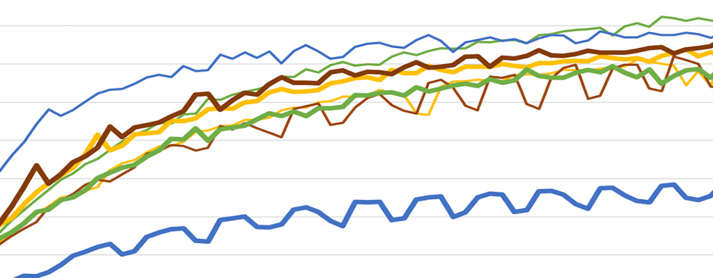
In the diagram below the number of threads is on the X axis. The thick lines (left hand scale) are thousands of TPS and the thin lines of the same color (right hand scale) are server side CPU. Because we scale by adding threads instead of aiming for a specific workload we see a distinctive curve.

Workload A
‘A’ is 50% Read and 50% write. In this configuration it flattens off around 350K operations per second because we saturate the underlying IO subsystem. Even though Volt Active Data is an in memory database we still have two forms of sequential IO. We snapshot the contents of RAM to disk at regular intervals and also stream incoming write requests to a ‘command log’. Because workload ‘A’ is the only write intensive workload it gets noticeably lower performance, as it’s the only workload to use the command log.
Workloads B, C & D
These workloads are either 95% read or 100% read. They all reached 375K TPS or more. Of the available 8 cores (4 from each server) we were using them in 8 groups of 2 for high availability purposes, with each pair doing the same work at the same time. That means that each core was handling around 46,875 transactions per second.
Workload E
Workload ‘E’ is tricky, as it returns 50 times more data than the other workloads, with each record being around 1KB, which has implications for both network and CPU costs.

We tested two implementations:
- ‘Scan’ does a globally read consistent query, in which all the nodes of the server cooperate to produce a result which is what you’d get if you had a single huge RDBMS. This is overkill for a lot of applications and a majority of YCSB implementations don’t do this.
- ‘ScanAll’ asks each partition inside Volt Active Data to query and sort its data and send the results back across the wire to the client, which then merges and prunes the data. It’s a lot more scalable but does not guarantee that each partition was queried at the exact same moment in time, although it’s a racing certainty the queries happen within a couple of milliseconds of each other.
At 5,500 TPS the ‘Scan All’ implementation’s client is reading about 275MB of data for each of 12 partitions per second (1K payload * 50 Rows per partition * 5,500 per second * 12 partitions), or around 3.2GB per second being sent to the client overall. Because of how Volt Active Data implements High Availability we also need to account for another 3.2GB of intra-cluster traffic. Given that the workload isn’t disk bound and that neither client nor server’s CPU exceed 15% during the tests , it’s reasonable to assume we ran out of network capacity, especially as AWS doesn’t give an SLA for network bandwidth for z1d.3xlarge, limiting itself to saying that z1d.3xlarge has “Up to 10,000 Mbps”
Latency
A lot of Volt Active Data’s customers are obsessed not just with millisecond latencies, but also by how consistently low latency is. For them a ‘long tail’ is a major problem. So traditionally a Volt Active Data benchmark involves running greater and greater workloads until target latency measured at the 99th percentile breaches some threshold. Below is a graph showing how average and 99th percentile latency behaves as the number of threads and TPS increases. While average latency slowly creeps about 0.8ms over time the 99th percentile latency both trends towards 3.5ms and increases noticeably faster. What we can say is that for workload ‘a’ latency is under 1ms until we get to around 170K TPS.

Bear in mind that all of this is on a generic AWS configuration, without making any heroic attempts to maximize performance. Our goal is to create something that people evaluating Volt Active Data can do for themselves. This is not – and does not claim to be – the ‘most’ Volt Active Data can get on this benchmark or on AWS.
A Comparison between YCSB and our Telco Charging Demo…
As I mentioned at the start of this post most Volt Active Data applications do far more work on the server side than at the client side, which is one of the reasons we didn’t get fully involved with YCSB earlier. We recently released an open source telco charging demo and accompanying blog post, which is a simplified implementation of the logic used by our customers to make prepaid mobile phones work. In the charging demo we got 22.5 K TPS per core on the same platform, versus 46.8K TPS per core in YCSB, but each charging demo event issues between 7 and 14 SQL statements per transaction instead of the one or two that YCSB does.
Thanks to Alex Rogers, who wrote our original implementation, and Sean Busbey, who helped shepard our implementation into the core YCSB repository.